Statistical Tools and their Usage – Regression Analysis

Regression analysis can be used to find out the relation between a set of variables statistically. This is done by identifying a curve or line that best fits the variables provided. Regression analysis is widely used in marketing research for trend analysis and for making predictions. In this article, we will be explaining simple linear regression only.

Case Based Explanation

Since it is inevitable to use numbers and perform some calculations to bring out the concept of regression, we will be demonstrating a case throughout the article to explain the statistical part in an easy way.

Suppose that after a few years of working in the industry, a person decides to go back to the university to get additional skills. Since education these days is expensive, the person would want to know whether education really increases the salary.

To start, we need to see how much wage is expected to increase with every additional year spent at the university. The intuitive way to go about it is to survey a sample of individuals and ask each of them how much they earn and how many years they have spent at school and then determine whether we can observe a pattern in their responses.

For the sake of simplicity and explanation, let’s say that we survey 10 individuals (In reality a much larger sample size is required to get reliable results). A random sample of 10 people will generate 10 data points. A scatter graph in excel is the best way to represent this.

Education is the independent variable depicted on the X axis and Wage is the dependent variable, to be plotted on the Y axis. The general pattern in the data set can be determined, i.e. relationship between wages and education can be obtained by the points on the scatter graph. For example, suppose that one person, referred to as P1, has 13 years of education and is earning $20 per hour. The next person, P2, has 20 years of education and paid $30 per hour.

Equation of a line is Υ = mX + b, where m is the slope and b is the intercept, i.e. where the line cuts the y axis. We have to find this line of best fit that will represent the general pattern in the sample.

In regression analysis, the line will be represented as Υ = β0+ β1X. We have simply changed the notation: β0 is the intercept and β1 is the slope of the gradient of the line. Software packages such as excel and MATLAB, can estimate the regression line.

So the equation now becomes:

Wages = β0 + β1Education

Situation 1

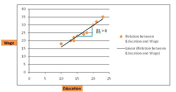
To determine whether there is a relation between wages and education, observe β1, the slope of the regression line. If β1 is positive, then there is a positive relation between wages and education. The more education a person attains, the higher the wage. This is clarified by the graph below:

Situation 2

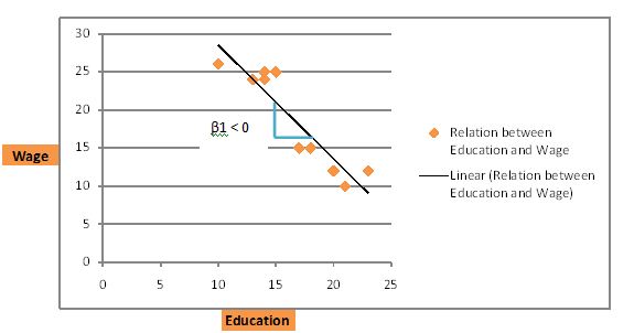
If the data from the survey looks like the graph below, a negative relation exists. The regression line is downward sloping from left to right. The trend here is that the more educated an individual, the less they earn in wages.

Situation 3

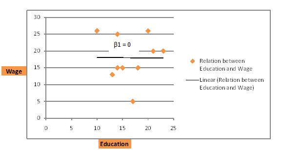
A third scenario is when there is no relation between wages and education. In that case, the line would cut through the data as follows; the line of best fit is a horizontal line.

Wages = 5 + 1Education

Suppose an individual has just finished high school and has 12 years of education. Substituting the value in the above equation, we get the hourly wage as:

Wages = 5 + 1×12 = 17

The next individual with 22 years of education, his expected wage would be:

Wages = 5 + 1×22 = 27, i.e. $27per hour.

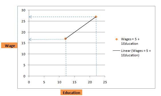
Thus we see that, for every additional 1 year of education, wages is expected to increase by $1 per hour. In case of a person with no education, β0 = 0, the equation reduces down to: wages = 5. This is the minimum wage since if a person has no education, he or she is expected to get at least $5 per hour.

Residuals

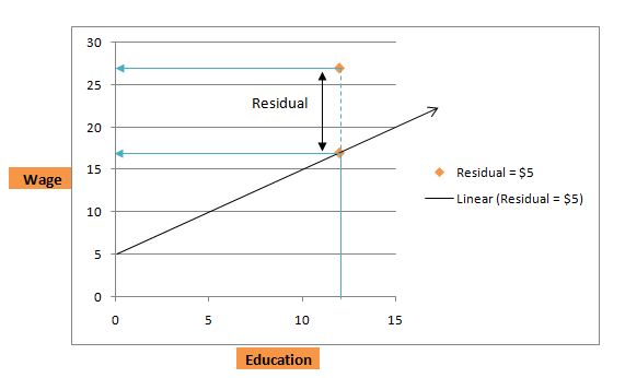
Referring to the equation of person P1 above with 12 years of education, the individual earns $17 per hour. However suppose in reality we find that the person actually earns $22 per hour! This does not imply that the regression equation is incorrect, but in fact can be attributed to a factor termed as residual. Thus residual is the difference between the actual wage and predicted wage.

So for P1, the residual is 22-17 = 5($). The regression model is the best guess at the hourly wage given the level of education. However, in real life many other factors in addition to education such as number of years of experience, IQ, networking ability, height, etc.

They were not accounted for and are contained in the residual term depicted by µ. So the revised equation would now be:

Υ = β0+ β1X + μ

Summary

The main highlights of the article above are as follows:

• The regression line is the line of best fit. It is the line that best represents the trend or relation in the given data
• β1 is the slope of the line. The relation between the dependent and independent variable is:
• Positive If: β1 > 0
• Negative If: β1 < 0
• No Relationship If: β1 = 0
• The estimated regression can be used to make predictions for Υ given X.
• Residual = Actual - Predicted
• The residual term accounts for the error in the prediction. It contains all other factors (except X) that impact Y.