


Economics
The Problem with REITs

February 7, 2025
 The World without Bankruptcy Laws
Bankruptcy is one of the natural states which a company may find itself in. Entrepreneurship is primarily about taking risks. When companies take risks, some of them succeed, whereas others fail. Hence failure is a natural part of the business. However, many critics of bankruptcy laws believe that there isn’t a need for an elaborate […]
The Wirecard and Infosys Scandals are a Lesson on How NOT to Treat Whistleblowers
What is the Wirecard Scandal all about and Why it is a Wakeup Call for Whistleblowers Anyone who has been following financial and business news over the last couple of years would have heard about Wirecard, the embattled German payments firm that had to file for bankruptcy after serious and humungous frauds were uncovered leading […]
Why the Digital Age Demands Decision Makers to be Like Elite Marines and Zen Monks
How Modern Decision Makers Have to Confront Present Shock and Information Overload We live in times when Information Overload is getting the better of cognitive abilities to absorb and process the needed data and information to make informed decisions. In addition, the Digital Age has also engendered the Present Shock of Virality and Instant Gratification […]
Why Indian Firms Must Strive for Strategic Autonomy in Their Geoeconomic Strategies
Geopolitics, Economics, and Geoeconomics In the evolving global trading and economic system, firms and corporates are impacted as much by the economic policies of nations as they are by the geopolitical and foreign policies. In other words, any global firm wishing to do business in the international sphere has to be cognizant of both the […]
Why Government Should Not Invest Public Money in Sports Stadiums Used by Professional Franchises
In the previous article, we have already come across some of the reasons why the government should not encourage funding of stadiums that are to be used by private franchises. We have already seen that the entire mechanism of government funding ends up being a regressive tax on the citizens of a particular city who […]
Suppose you are an HR professional and want to determine:
All these are routine scenarios in an organization. But their impact is huge. How, as an HR professional, can you determine which variables have what impact on employee productivity?
Regression analysis offers you the answer. It helps you explain the relationship between two or more variables.
With Explanation Comes Consideration!
However, before we go into details and understand how regression models can be employed to derive a cause and effect relationship, there are several important considerations to take into account:
Regression analysis simplifies some very complex situations, almost magically. It helps researchers and professionals correlate intertwined variables. Linear regression is one of the simplest and most commonly used regression models. It predicts the cause and effect relationship between two variables.
The model uses Ordinary Least Squares (OLS) method, which determines the value of unknown parameters in a linear regression equation. Its goal is to minimize the difference between observed responses and the ones predicted using linear regression model. There are certain requirements that you need to fulfill, in order to use this model. Otherwise the results can be confusing and ambiguous.
Let’s understand it with the help of an example:
The phenomenon is: Work experience and remuneration are related variables. The linear regression model can help predict the remuneration slab of an employee given his/her work experience.
Now the problem arises how to represent it statistically.
There are two lines of regression – Y on X and X on Y.
Y on X is when the value of Y is unknown. X on Y is when the value of X is unknown.
Here are their statistical representations:
Suppose, the value of remuneration is = Y and the value of experience is = X
|
Selection of Line of Regression
The statistical representation above is an example to show how to develop econometric models when the value of one of the variables is known and another’s unknown. However, this doesn’t mean that both the representations are correct.
This is because remuneration may depend on the work experience of an individual but the vice versa is not true. Experience doesn’t depend on remuneration. Therefore, you’ll have to carefully choose the dependent variable and then the line of regression.
A linear regression equation shows the percentage increase or decrease in the value of dependent variable (Y) with the percentage increase or decrease in the value of independent variable (X).
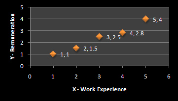
Let us suppose the values of X and Y are known.
Table 1
| X | Y |
| 1 | 1 |
| 2 | 1.5 |
| 3 | 2.5 |
| 4 | 2.8 |
| 5 | 4 |
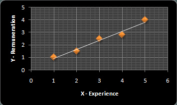
Graphically it’s represented as:
The white line connecting all the dots in the graph above represents the error or prediction. But you now want to find the best-fitted line of regression to minimize the error of prediction. The aim is to help find the best-fitted line of regression.
How to Find the Best-Fitted Line of Regression?
By using the ordinary least squares method!
Let us continue with the above example:
Table 2
| X | Y | XY | X-X’ | Y-Y’ | (X-X’)(Y-Y’) | (X-X’)2 | (Y-Y’)2 | |
| 1 | 1 | 1 | -2 | -1.16 | 2.32 | 4 | 1.346 | |
| 2 | 1.5 | 3 | -1 | -0.66 | 0.66 | 1 | 0.436 | |
| 3 | 2.5 | 7.5 | 0 | 0.34 | 0.34 | 0 | 0.116 | |
| 4 | 2.8 | 11.2 | 1 | 0.64 | 0.64 | 1 | 0.410 | |
| 5 | 4 | 20 | 2 | 1.84 | 3.68 | 4 | 3.386 | |
| Sum | 15 | 10.8 | 42.7 | 7.64 | 10 | 5.69 | ||
| Mean | X’ = 3 (15/5) | Y’ = 2.16 (10.8/5) |
The primary equation is:
Y = a + b(X) +e (error term)
In this case, e is zero because it is assumed that the independent variable (X) has negligible errors.
Therefore, it remains Y = a + b(X).
Let us now find the value of b.
b = [ ∑ XY – (∑Y)(∑X)/n ] / ∑(X-X’)2
Substitute the values in the above formula:
b = [ 42.7 – (15*10.8)/5 ]/10 = [ 42.7 – 162/5 ]/10 = [ 42.7 – 32.5 ]/10 = 10.2/10 = 1.02
b = 1.02
Therefore,
a = Y – b(X)
a = Y – 1.02(X) or a = ∑Y/n – 1.02 (∑X/n)
a = 2.16 – 1.02*3 = 2.16 – 3.06
a = -1.06
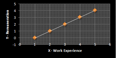
By substituting the value of a, b and X, we can find the corresponding value of Y.
Y = a + b(X) = -1.06 + 1.02X
When X = 1
Y = -1.06 + 1.02*1 = -0.04
When X = 2
Y = - 1.06 + 1.02*2 = 0.98
When X = 3, Y will be 2
When X = 4, Y will be 3.02
When X = 5, Y will be 4.04
Table 3
| X | Y |
| 1 | -0.04 |
| 2 | 0.98 |
| 3 | 2 |
| 4 | 3.02 |
| 5 | 4.04 |
The best-fitted regression line will be:
Properties of the Best-Fitted Regression Line/Estimators
Whenever you use a regression model, the first thing you should consider is – how well an econometric model fits the data or how well a regression equation fits the data.
This is where the concept of coefficient of determination comes in. The regression models are generally fitted using this approach.
It determines the extent to which dependent variable can be predicted from independent variable. It assesses the goodness-of-fit of the Ordinary Least Square Regression Model.
Denoted by R2, its value lies between 0 and 1. When:
Higher the value of R2, better fit the model is to the data.
Let’s now understand how to calculate R2. The formula for finding R2 is:
R2 = { (1 / n) * ∑ (X-X’) * (Y-Y’) } / (σx * σy)2
Where n = number of observations = 5
∑ (X-X’) * (Y-Y’) = 7.64 (Ref Table 2)
σx is the standard deviation of X and σy is the standard deviation of Y
σx = square root of ∑ (X-X’)2/n = √10/5 = √ 2 = 1.414
σy = square root of ∑ (Y-Y’)2/n = √5.69/5 = √1.138 = 1.067
Now let’s determine the value of R2
R2 = { 1/5 (7.64) } / (1.414 * 1.067)2 = 1.528 / (1.509)2 = 1.528/2.277 = 0.67
Hence R2 = 0.67
Higher the value of coefficient of determination, lower the standard error. The result indicates that about 67% of the variation in remuneration can be explained by the work experience. It shows that the work experience plays a major role in determining the remuneration.
Properties of Estimators
The linear regression model is used when there is a linear relationship between dependent and independent variables. When the value of a dependent variable is based on multiple variables (more than one), we use multiple regression analysis. We’ll study about this in the next article. Stay tuned!

Your email address will not be published. Required fields are marked *
The Problem with REITs
February 7, 2025
What is Seasonal Employment and How to Manage it ?
February 7, 2025
Social Evil #1: War and GDP
February 7, 2025